Measuring model complexity – Part 2: Putting theory into practice

In our previous blog post, we laid the groundwork for a complexity analyser by identifying key metrics for quantifying the complexity of workflow models. Now, we will focus on how to transform this theoretical foundation into actionable insights.

From metrics to complexity levels

The goal is to classify models into categories of low, medium, and high complexity. This is a typical use case for unsupervised machine learning, particularly clustering algorithms. The underlying assumption is that models with similar complexity metrics will naturally fall into distinct groups. For instance, simpler models are likely to have lower NOAJS and CFC, while more complex models tend to have higher values for these metrics due to the increased use of gateways. With this in mind, the K-Means algorithm was selected for clustering.

Preparing the dataset

As a product and consultancy provider, we have access to a vast repository of orchestration models. Our dataset comprised real-world use cases and demo applications created by seasoned modelers, spanning a variety of domains such as medical, infrastructure, finance, and manufacturing. Ultimately, the dataset included:

• 25 applications

• 332 BPMN processes

• 54 CMMN cases

A quick review of these models revealed diverse modeling styles, such as:

1. Cases invoking multiple small processes.

2. Applications with large BPMN processes but no CMMN cases.

3. Processes combining event-subprocesses and call activities, without CMMN cases.

4. Large CMMN cases with multiple event listeners.

Satisfied with the dataset’s diversity, the next step was to clean and prepare the data for analysis.

Data cleaning and normalization

Like any machine learning pipeline, data cleaning was essential. Initially, processes with only one activity seemed like outliers worth removing. However, upon closer inspection, these were often purposeful, serving as delegate processes for tasks like data cleaning or sending emails. Recognizing their significance, these were retained.

The next step was normalizing the metrics to ensure fair contribution across all dimensions. Without normalization, metrics like NOAJS, which range from 0 to infinity, could dominate over metrics like density, which always fall between 0 and 1. A Min-Max normalizer was used to scale all values between 0 and 1, ensuring a balanced input for clustering.

K-means clustering approach

For the initial clustering, the algorithm was configured to create three clusters corresponding to low, medium, and high complexity. K-means requires defining the number of clusters beforehand, and while methods like the elbow method can help determine the optimal number, our focus was on these three levels. Importantly, the algorithm was left to assign clusters without any manual intervention to avoid bias.

The pipeline for clustering was as follows:

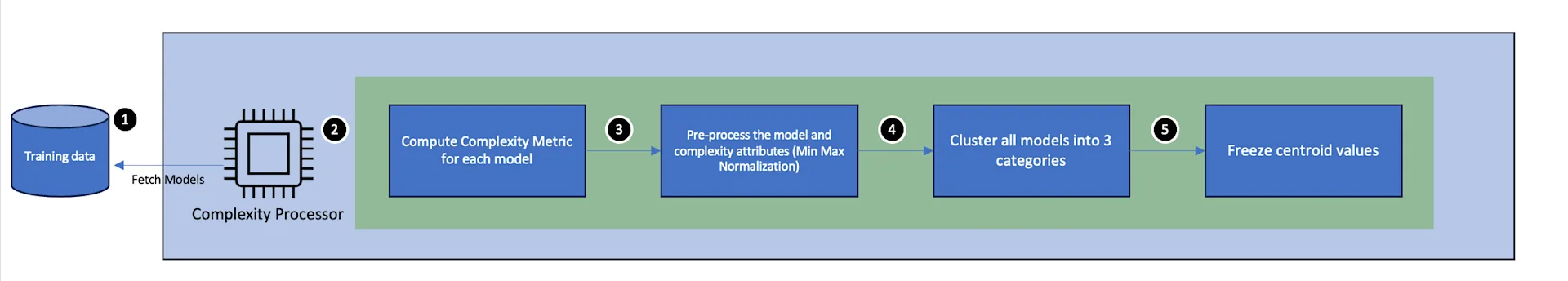
Figure 1 : Clustering Pipeline

1. Fetch all BPMN and CMMN models from the dataset.

2. Calculate metric values for each model.

3. Normalize the metrics using Min-Max scaling.

4. Apply K-Means to classify models into three clusters.

Challenges with K-means labelling

A limitation of K-Means is its inability to assign cluster labels based on predefined criteria (e.g., low, medium, high complexity). While initial cluster centroids could be provided to influence clustering, this would compromise the algorithm's independence. Instead, the task of interpreting and labelling clusters was handled post-clustering.

To validate the clustering results, a graph plotting NOAJS vs. CFC was created. This visualization provided a clearer understanding of how the models were distributed across the complexity spectrum, offering insights into the validity of the clusters.

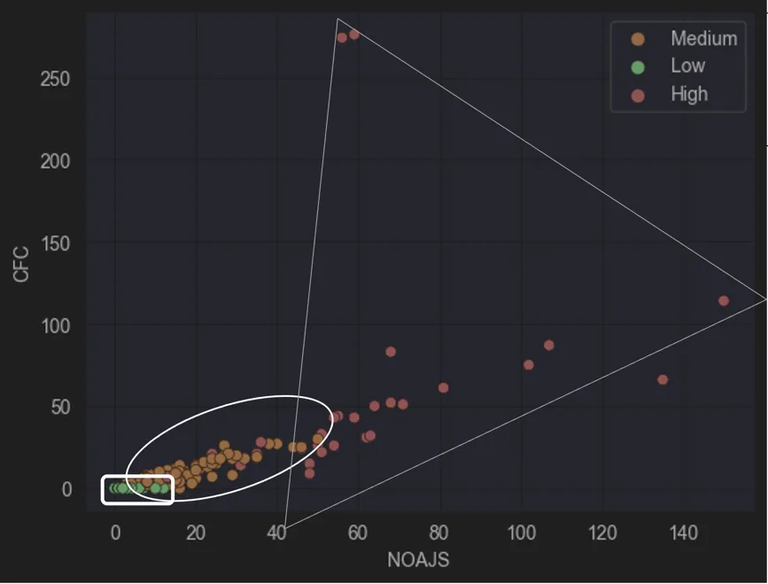
Figure 2 : CFC vs NOAJS

Analysing the graph, three distinct clusters emerged:

1. Models with 0 CFC and < 18 NOAJS

2. Models with < 40 CFC and < 50 NOAJS

3. All remaining models

Based on the initial hypothesis- that low-complexity models typically have no gateways and a smaller number of activities - the first group was classified as low complexity. The second and third groups, showing progressively higher values for both metrics, were labelled as medium complexity and high complexity, respectively.

This classification aligns with the expectation that as model complexity increases, the use of gateways and activities becomes more pronounced, resulting in higher CFC and NOAJS values.

Interpreting the results

With the clusters defined, the next step was to explore which metrics contributed most significantly to model complexity.

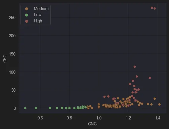
Figure 3: CFC vs CNC

1. Contribution of CFC (Control Flow Complexity) to the complexity As anticipated, models with CFC = 0 were classified as low complexity. However, two models with CFC = 0 ended up in the medium complexity group. Upon further analysis, these models exhibited high CNC values and referenced more than ten other models, highlighting additional dimensions of complexity beyond control flow.

2. CNC as a Key Factor in Low Complexity Models CNC (Coefficient of Network Connectivity) emerged as a defining factor for low-complexity models. Simple models tend to have low CNC values since increasing CNC generally requires more sequence flows per node, often achieved by adding gateways. This aligns with our previous graph, further validating CNC as a robust indicator of complexity.

3. Models with NOAJS (Number of Activities, Joints and Splits) > 60 Are Very Complex This was an expected result. Any model with NOAJS > 60 signals a need for decomposition into smaller subprocesses. High NOAJS values tend to clutter the model, making it harder to read and maintain.

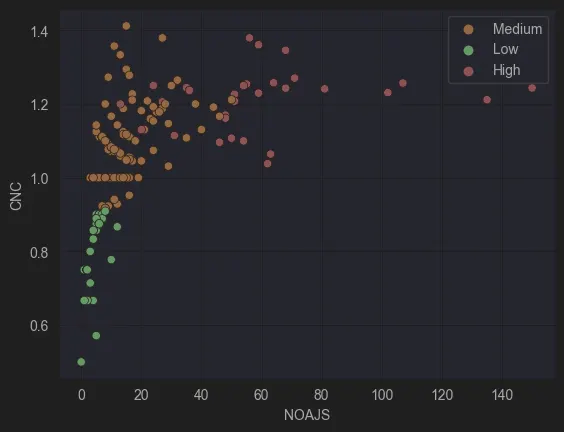
Figure 4: CNC vs NOAJS

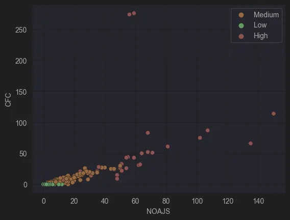
Figure 5 : CFC vs NOAJS

4. Contribution of NVAR

To analyze NVAR (Number of Variables) as a contributing factor, we observed an interesting trend in the graph:

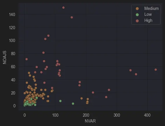
Figure 6: NOAJS vs NVAR

Models classified as complex generally followed a curve around the intersection of NVAR and NOAJS. If either metric approached its maximum, the model was consistently classified as complex. This trend held true for both BPMN and CMMN models, where complexity metrics accounted for the weighted sum of modelling elements.

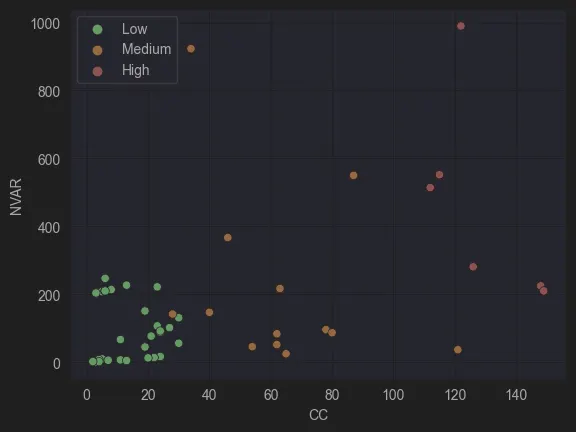
Figure 7: NVAR vs CC

5. Role of NRC in Model Complexity

NRC (Number of Referenced Children) plays a significant role in both BPMN and CMMN models. Complex models often incorporate multiple modelling components or call numerous subprocesses or subcases.

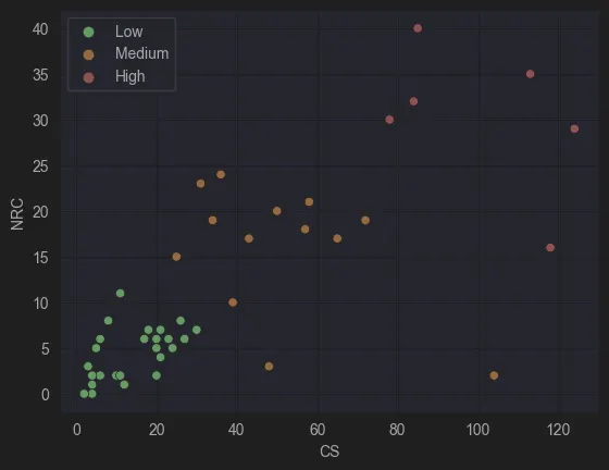
Figure 8: NRC vs CS

However, NRC isn’t the sole determinant. Poorly designed models might consolidate everything into a single, bloated process without invoking subprocesses, thereby reducing NRC while maintaining high complexity.

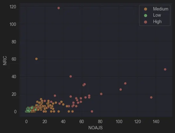
Figure 9: NRC vs NOAJS

Should NRP Be Included?

NRP (Number of Referencing Parents) posed an interesting challenge. Initially, this metric wasn’t included in clustering. However, in BPMN models, some workflows seemed more critical at the application level but were classified as low or medium complexity. The assumption was that critical workflows would be reused by multiple other processes or cases, warranting their inclusion in the analysis. From the perspective of identifying models for refactoring, this might not be universally agreed upon, but for evaluating critical models, including NRP yielded insightful results.

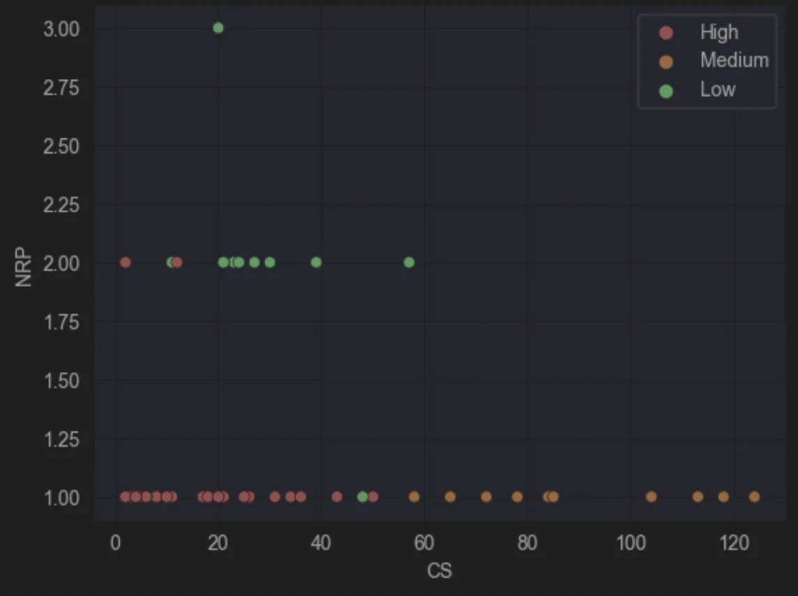
Figure 10: NRP vs CS

When applied to CMMN models, however, NRP disrupted the clustering algorithm. This was expected since CMMN cases often act as the central orchestration layer, calling various subprocesses. In the sample dataset, NRP values were mostly low, with few exceptions, leading to high entropy in clustering. Ultimately, it made sense to exclude NRP from CMMN clustering.

This analysis highlighted the limitations of relying solely on standard metrics. While traditional studies often focus on individual BPMN or CMMN models, real-world deployment units - such as those in Flowable - are far more complex. These units include cases, processes, forms, DMNs, and other components. By incorporating additional metrics such as NRP (Number of Parents), NRC (Number of Children), and NVAR (Number of Variables), a more comprehensive framework for evaluating real-world model complexity was developed. The study began as a question about workflow complexity and ultimately provided a robust framework for categorizing and understanding diverse models.

In the final part of this series, we’ll look at how the Complexity Analyzer can evolve from a diagnostic tool into a catalyst for smarter, more collaborative, and data-informed workflow design.